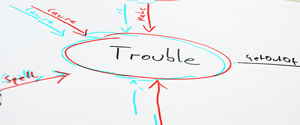

As an anti-virus vendor, we analyse several hundred thousand of potential malware samples per day. We have to classify these new samples which means first of all that we simply have to decide whether the sample is benign or malicious. In case it is malicious, we want to know whether it belongs to a malware family we already know or whether it is a completely new malware. When the malware sample is completely new then a human analyst should probably take a look at it and create a new detection. In case it belongs to an already known family, we improve the family’s detection if necessary to also detect the new sample.
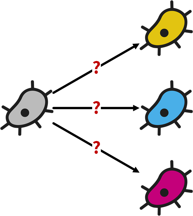
Malware families consist of malware samples that share the same behaviour and that also have mostly the same code. Their authors simply change parts of the binary in order to avoid detections by static signature-based scanners. This can, for example, simply be done by using a different packer. So, the malware samples that belong to the same family look different on disk, but still exhibit the same behaviour. We want to use this fact for our classification as it allows us to assign malware samples to known families based on their behaviour.
The behaviour of malware samples can be represented by features. The IP address of a contacted host is for example such a feature, the name of a created file is another. This leads us to the question of how we can find malware samples that have a lot of features in common as that likely means that the samples belong to the same malware family.
This article is part of a series on graph databases
In this series we take a look at how you can use a graph database in the context of malware analysis:
- Malware analysis with a graph database (this post)
- How to avoid doppelgängers in a graph database
- One graph to find them all - How to find similar malware samples
- Graph databases: Bad neighborhoods, parents and machine learning - Malware classification
Why Use a Graph Database for Malware Analysis?
A graph database is a database that models data in a graph which consists of vertices and edges. Vertices and edges can typically have properties and an edge connects two vertices with each other. Edges are treated as “first class citizen” in a graph database which reflects the importance of modelling relationships in a graph database. This model makes graph databases a good choice for use cases where it is important to find relationships, especially when the relationships are more complex because they require traversing over multiple edges. Relational databases by contrast need computational expensive joins to query relationships.
Since finding relationships between malware samples is exactly the problem we are trying to solve, a graph database is a natural fit for our use case. We just need to create the graph with samples and their features in a way that allows us to find relationships between samples based on their shared features.
Choosing a Graph Database
Good support for the Apache TinkerPop framework was the most important requirement for our choice of the graph database system to use because TinkerPop is the de facto standard for graph databases and graph computing. Using a TinkerPop enabled database means that we avoid a vendor lock-in as we could easily switch to another TinkerPop enabled database and also that we profit from TinkerPop’s growing ecosystem. Another important requirement for us was horizontal scalability. These two main criteria led us to the JanusGraph database, a graph database hosted at the Linux Foundation.
Both of these projects, Apache TinkerPop and JanusGraph, are not only open-source projects but they are also backed by an open community which was another important decision point for us. We now contribute to both projects on a regular basis, not only to implement features that are important for us but also because we want to see these projects and their communities grow. A healthy and growing community usually results in a growing ecosystem which includes new libraries and tools that could also be helpful for us at some point.
Another nice advantage of JanusGraph is also that its storage and index backends are pluggable. This allowed us already to migrate from Apache Cassandra to the easier to configure ScyllaDB. It may also provide a way forward towards a graph database that is not only scalable but that also offers ACID transactions with a backend based on FoundationDB for which a first JanusGraph storage adapter already exists.
Creating a Malware Feature Graph
Now that we have established why we want to use a graph database for malware analysis, we can discuss how we extract the features and how we store them in our graph database. The following diagram gives an overview of our analysis system that fills our graph database:
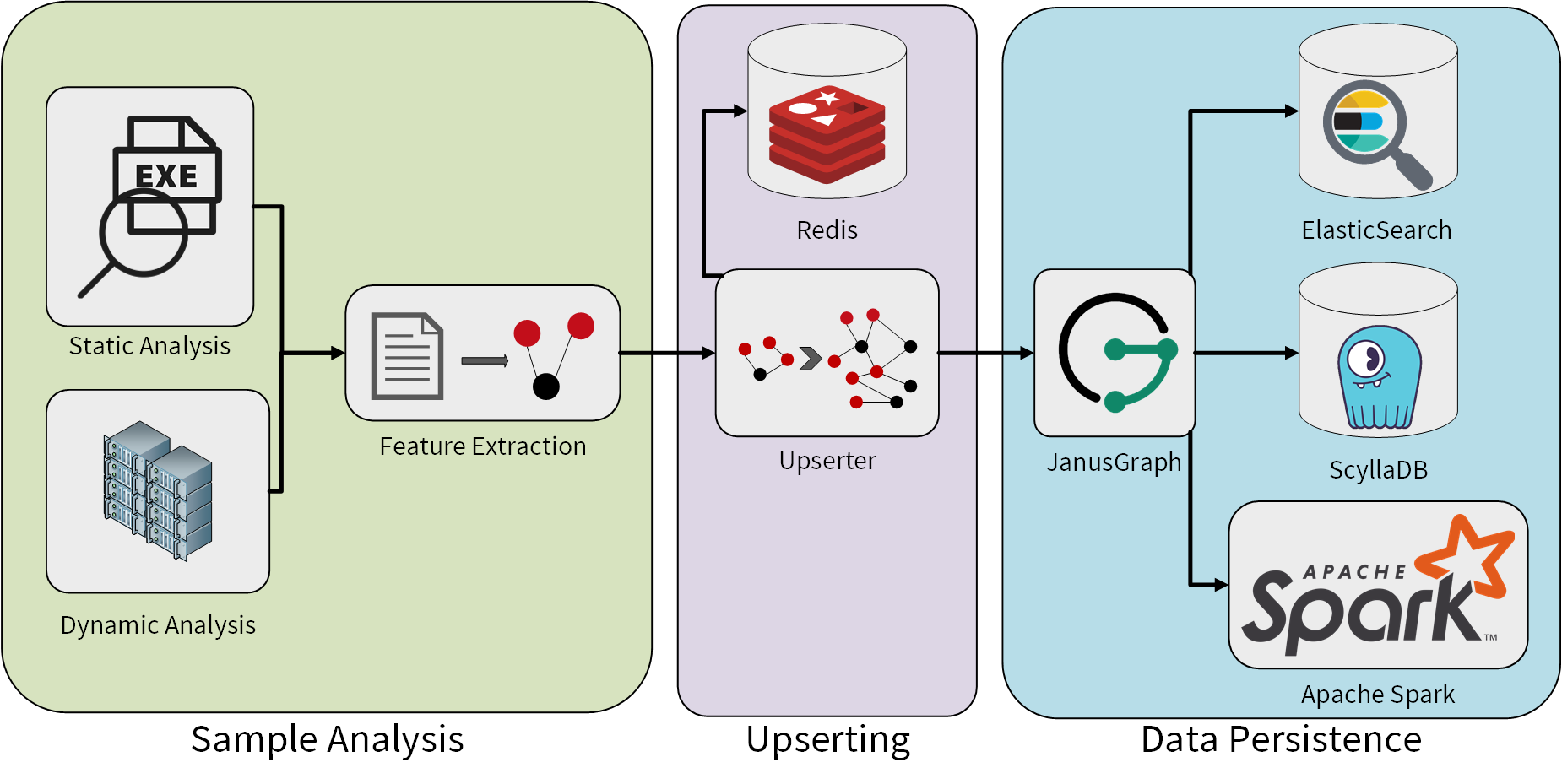
The sample analysis uses static and dynamic analysis to extract as much information as possible from a malware sample. Dynamic analysis means in this context the execution of the malware sample in a sandbox with the subsequent analysis of the observed behaviour. This includes for example the analysis of recorded network traffic which can give us an insight into the command and control (C&C) infrastructure of the malware.
For each sample we process, our feature extraction creates a small graph. The sample is represented by a vertex and connected to feature vertices by edges in this graph. The following figure shows how such a small graph can be created based on information about an API call the malware made:
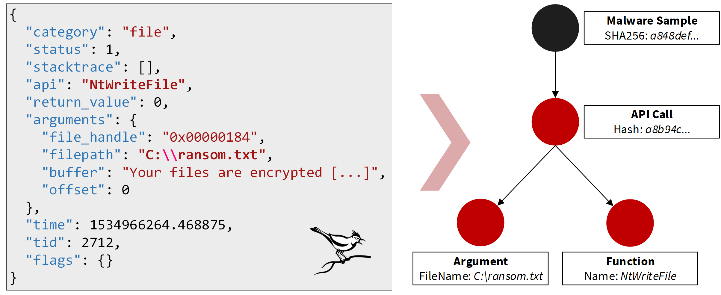
The JSON document shown in the figure is an excerpt of an API trace created by the open-source Cuckoo sandbox1. The full API trace contains information about all calls to the operating system API observed during the sandbox run. The shown API call tells us that the malware wrote into a file with the path C:\ransom.txt by calling NtWriteFile which already indicates that the malware could be a ransomware as the created file appears to be a ransom note. (This is also confirmed by the content of the created file that starts here with “Your files are encrypted”). The graph representation of this API call consists of three vertices in our model. One vertex aggregates the whole API call and is connected by two outgoing edges to vertices that represent the API function NtWriteFile that was called and the filename as the interesting argument. Another vertex then represents the malware sample and is connected with an edge to the aggregate API call vertex. This gives us a small graph to represent the information we can extract about the malware based on this API call. We follow a similar approach for all features we can observe. This results in a lot of small graphs for each malware sample we analyse.
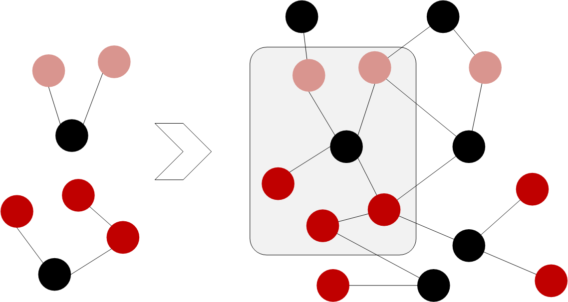
All such small graphs are upserted into our graph database. This creates a big graph with information about all malware samples we have analysed. Malware samples which share common features are connected by those features as their common neighbours in the big graph. These common neighbours make it easy to find similar malware samples. One simply has to traverse from the sample over its features to other samples that have the same features.
Our upserting process that fills the graph uses a Redis in-memory database as a lock manager for this task to avoid getting duplicates in the graph when multiple threads try to upsert the same data in parallel. Since upserting of data while avoiding duplicates in a graph database is a frequent requirement, we will describe this process in greater detail in a follow-up blog post.
Apart from the already mentioned components, the data persistence layer also consists of an Elasticsearch cluster and, if needed for a specific use case, Apache Spark. Elasticsearch allows us to use full-text searches in our Gremlin traversals, e.g., to find IP addresses in a certain range. Apache TinkerPop (and therefore JanusGraph as it is TinkerPop-enabled) not only provides capabilities to perform real-time OLTP traversals, but also offers an integration with Apache Spark to perform long running OLAP operations that can work on all data stored in the graph in parallel. We can use that for example in the context of classification of malware where existing classifications of malware samples are used to classify yet unknown samples based on features they have in common.
Upserting
Upserting describes an operation that inserts data into a database if it does not exist already or updates the existing data otherwise. The term upsert is a portmanteau of update and insert.
OLTP and OLAP
OLTP stands for online transaction processing and describes systems that can answer a large number of short transactions, e.g., to retrieve a data record from a database. Online analytical processing (OLAP) on the other hand describes systems that handle longer running operations that typically affect a large number of data records in the database. OLAP system can for example be used for machine learning.
Conclusion
A graph is a natural representation of the domain model in the context of malware analysis. Using a graph database to store the features we have extracted during the analysis of malware samples allows us to find relations between similar samples based on the features they have in common. We will take a look at use cases where these relations are important in follow-up blog posts.
1 We are using a sandbox system developed in-house that creates API traces in a different format. The API traces created by Cuckoo are only used as an example here.